
TIPMIP-ICE SHEETS aims to systematically explore ice-sheet tipping risks in Greenland and Antarctica across multiple ice-sheet models, based on the TIPMIP framework (Winkelmann et al., in review). In the following, we summarize the TIPMIP-ICE SHEETS experimental protocol (Winkelmann/Klose et al., in prep.).
Icesheet Domain Leads





Protocol
Last update: 17 September 2026
Overall, we expect participating ice-sheet models to fulfill a number of high-level features which are needed to study ice-sheet tipping dynamics:
- The present-day ice sheets on Greenland and in Antarctica are not in steady state. The initial ice-sheet state for the TIPMIP-ICE SHEETS simulations should either be interpretable as pre-industrial state or overall capture the observed mass imbalance in the present-day. In addition, if interpreted as a pre-industrial state, a pre-industrial control simulation should not show substantial retreat (or collapse).
- We expect participating ice-sheet models to represent the surface melt-elevation feedback.
- A representation of the response of the solid Earth to ice-sheet changes is required for participation in TIPMIP-ICE SHEETS.
- Ice-sheet models participating in TIPMIP-ICE SHEETS should represent calving from a freely retreating ice front.
Please find further details and examples on how to implement these high-level features in the ice-sheet models below.
Beyond fulfilling these high-level features, the TIPMIP-ICE SHEETS experimental protocol adopts an open approach. This includes ice-sheet model input data / boundary conditions (e.g. geothermal heat flow), and, in particular, applies to the translation of changes in climate provided by TIPMIP-ICE SHEETS to the ice-sheet model forcing. The open approach aligns well with the ISMIP7 protocol, allowing ice-sheet modelling groups to use the same or at least very similar ice-sheet model setup for both model intercomparisons.
TIPMIP-ICE SHEETS experiments are organized in three Tiers. Participation in TIPMIP-ICE SHEETS requires running at least the experiments in Tier 1, which sum up to 1800 – 10400 model years. We encourage participating ice-sheet modelling groups to run as many additional experiments as possible in Tier 2 and 3 with a total of 20800 model years in each Tier.
Contact
TIPMIP-ICE SHEETS Domain Leads: icesheets@tipmip.org
TIPMIP Icesheets Listserv: tipmip-icesheets-wg@listserv.dfn.de
Timeline
08.2026 Ice-sheet model forcing available via DKRZ (see Data access and distribution)
End of 10.2026 Submission of ice-sheet model contributions (at least Tier 1 to be part of the first multi-model analysis papers)
List of experiments
The TIPMIP-ICE SHEETS protocol (Winkelmann/Klose et al., in prep.) includes three types of experiments (Fig. 1) based on the overarching TIPMIP experimental design (Winkelmann et al., in review):
- Climate ramp-up from pre-industrial climate to 4°C global warming
- Climate stabilization at 2°C and 4°C global warming
- Climate reversal (“drop down” directly instead of ramp-down) to 2°C global warming and to pre-industrial climate
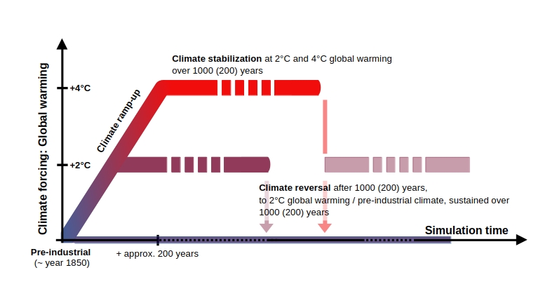
Using these experiments, the aim of TIPMIP-ICE SHEETS is to quantify the likelihood of crossing critical thresholds, the resulting committed ice-sheet changes and their reversibility. Different sources of uncertainty are systematically explored across three Tiers (see Table 1 and 2).
Climatic boundary conditions for each type of experiment are based on output from Earth System Models in TIPMIP-ESM (Jones et al., in review). TIPMIP-ICE SHEETS provides a set of variables suitable for translating the changes in climate to the ice-sheet models within the open approach, see Atmospheric forcing and Ocean forcing for details. Since TIPMIP-ESM focuses on timescales up to 200 years, a forcing extension is needed for the climate stabilization experiments in TIPMIP-ICE SHEETS. In particular, for the climate stabilization experiments, the first 50 years of the respective TIPMIP-ESM output are randomly sampled (with same random sampling for all ice-sheet models). Due to the large file size up to 1000 years of forcing for the climate stabilization and reversal experiments, the extended forcing is not directly available for download. Instead, Python scripts are provided that allow the ice-sheet modelling groups to generate the extended forcing after the download (see Data access and distribution).
Tier 1 covers an idealized climate ramp-up, stabilization and reversal as listed above. Participation in TIPMIP-ICE SHEETS requires running the full set of experiments with (at least) one ice-sheet model setup. Here, ice-sheet model setup refers to one set of “parameters” (e.g. friction law, friction law exponent) and fixed boundary conditions (e.g. geothermal heat flux, atmospheric/ocean climatology). Any change in parameters is considered as a distinct ice-sheet model setup. The changes in climate are based on output from a recommended Earth System Model from TIPMIP-ESM (Röntgen et al., in prep.). Tier 1 focuses on quantifying the ice-sheet tipping risks across as many individual ice-sheet models as possible (uncertainties in the ice-sheet model structure).
The climate ramp-up experiment spans a period of approx. 200 years, depending on the ESM (see Table 1 and 2) and the ice-sheet model initialization (see below). The climate stabilization and reversal experiments should ideally be run over 1000 years – if this is computationally not feasible, we have included an option to only run the stabilization experiment over 200 years and reverse thereafter (see Table 1 and 2). We also encourage modelling groups to run the reversal after 200 years as an additional experiment even when the reversal after 1000 years is possible.
Tier 2 experiments quantify uncertainties in key processes and feedbacks associated with ice-sheet tipping dynamics by repeating the set of experiments in Tier 1 with different model parameters. In particular, we ask each modelling group to choose parameter values representing
- a lower and higher strength of the surface melt – elevation feedback (e.g. atmospheric lapse rate in a lapse rate correction of the near-surface air temperature with changes in ice-sheet geometry, see Atmospheric forcing), compared to the ice-sheet model setup submitted in Tier 1.
- a lower and higher sub-shelf / frontal melt sensitivity for the Antarctic / Greenland Ice Sheet compared to the ice-sheet model setup submitted in Tier 1.
Uncertainty ranges for these key processes and feedbacks can be obtained from the references given in Atmospheric forcing and Ocean forcing.
Tier 3 samples uncertainties in the regional climate simulated by the TIPMIP ESMs. Three TIPMIP ESMs have been chosen to cover a wide range of atmospheric-to-oceanic warming trajectories in Greenland and Antarctica under the same change in global mean warming during the climate ramp-up experiment (Röntgen et al., in prep.).
We encourage the participating ice-sheet modelling groups to run as many Tier 2 and Tier 3 experiments as possible. For modeling groups running the Tier 1 climate stabilization and reversal experiments over 200 years only due to computational constraints, we still welcome submissions of Tier 2 and 3 experiments over this shorter timescale (even if not listed in Table 1 and 2 explicitly). We also welcome submissions exploring additional sources of uncertainty (such as parametric uncertainty associated with ice-sheet dynamics, initial state uncertainty, …). We are happy to coordinate across modelling groups to align ensemble designs. If such an uncertainty analysis is planned, we encourage modelling groups to email us (see Contact).
Table 1: List of TIPMIP-ICE SHEETS experiments (Tiers 1–3) for Antarctic Ice Sheet.
| Tier | Experiment | Ice-sheet model setup | ESM forcing | Length of experiment (in model years) | |
| Tier 1 | Exp01-NorESM2-LM-ramp-def | Ramp-up to 4°C | Default | NorESM2-LM | 207 |
| Exp01-NorESM2-LM-stab2.0-def | Stabilization at 2°C (simulation year 101 during ramp-up), ideally over 1000 years (if that is computationally not feasible, over 200 years) | 1000 (or 200) | |||
| Exp01-NorESM2-LM-stab2.0-200y-revpi-def | Reversal after 200 years from 2°C to pre-industrial | 1000 (or 200) | |||
| Exp01-NorESM2-LM-stab2.0-1000y-revpi-def | Reversal after 1000 years from 2°C to pre-industrial (if Exp01-NorESM2-LM-stab2.0-def was run over 1000 years) | 1000 | |||
| Exp01-NorESM2-LM-stab4.0-def | Stabilization at 4°C (simulation year 207 during ramp-up), ideally over 1000 years (if that is computationally not feasible, over 200 years) | 1000 (or 200) | |||
| Exp01-NorESM2-LM-stab4.0-200y-rev2.0-def | Reversal after 200 years from 4°C to 2°C | 1000 (or 200) | |||
| Exp01-NorESM2-LM-stab4.0-1000y-rev2.0-def | Reversal after 1000 years from 4°C to 2°C (if Exp01-NorESM2-LM-stab4.0-def was run over 1000 years) | 1000 | |||
| Exp01-NorESM2-LM-stab4.0-200y-revpi-def | Reversal after 200 years from 4°C to pre-industrial | 1000 (or 200) | |||
| Exp01-NorESM2-LM-stab4.0-1000y-revpi-def | Reversal after 1000 years from 4°C to pre-industrial(if Exp01-NorESM2-LM-stab4.0-def was run over 1000 years) | 1000 | |||
| Exp01-ctrl | Pre-industrial ctrl | 2200 (or 600) | |||
| Tier 2 Parametric uncertainty related to feedbacks | Exp02-NorESM2-LM-ramp-LowAtm | Ramp-up to 4°C | Lower atmospheric lapse rate | NorESM2-LM | 207 |
| Exp02-NorESM2-LM-stab2.0-LowAtm | Stabilization at 2°C (simulation year 101 during ramp-up) over 1000 years | 1000 | |||
| Exp02-NorESM2-LM-stab2.0-1000y-revpi-LowAtm | Reversal after 1000 years from 2°C to pre-industrial | 1000 | |||
| Exp02-NorESM2-LM-stab4.0-LowAtm | Stabilization at 4°C (simulation year 207 during ramp-up) over 1000 years | 1000 | |||
| Exp02-NorESM2-LM-stab4.0-1000y-rev2.0-LowAtm | Reversal after 1000 years from 4°C to 2°C | 1000 | |||
| Exp02-NorESM2-LM-stab4.0-1000y-revpi-LowAtm | Reversal after 1000 years from 4°C to pre-industrial | 1000 | |||
| Ex03-NorESM2-LM-ramp-HighAtm | Ramp-up to 4°C | Higher atmospheric lapse rate | 207 | ||
| Ex03-NorESM2-LM-stab2.0-HighAtm | Stabilization at 2°C (simulation year 101 during ramp-up) over 1000 years | 1000 | |||
| Ex03-NorESM2-LM-stab2.0-1000y-revpi-HighAtm | Reversal after 1000 years from 2°C to pre-industrial | 1000 | |||
| Ex03-NorESM2-LM-stab4.0-HighAtm | Stabilization at 4°C (simulation year 207 during ramp-up) over 1000 years | 1000 | |||
| Ex03-NorESM2-LM-stab4.0-1000y-rev2.0-HighAtm | Reversal after 1000 years from 4°C to 2°C | 1000 | |||
| Ex03-NorESM2-LM-stab4.0-1000y-revpi-HighAtm | Reversal after 1000 years from 4°C to pre-industrial | 1000 | |||
| Exp04-NorESM2-LM-ramp-LowOcn | Ramp-up to 4°C | Lower sub-shelf melt sensitivity | 207 | ||
| Exp04-NorESM2-LM-stab2.0-LowOcn | Stabilization at 2°C (simulation year 101 during ramp-up) over 1000 years | 1000 | |||
| Exp04-NorESM2-LM-stab2.0-1000y-revpi-LowOcn | Reversal after 1000 years from 2°C to pre-industrial | 1000 | |||
| Exp04-NorESM2-LM-stab4.0-LowOcn | Stabilization at 4°C (simulation year 207 during ramp-up) over 1000 years | 1000 | |||
| Exp04-NorESM2-LM-stab4.0-1000y-rev2.0-LowOcn | Reversal after 1000 years from 4°C to 2°C | 1000 | |||
| Exp04-NorESM2-LM-stab4.0-1000y-revpi-LowOcn | Reversal after 1000 years from 4°C to pre-industrial | 1000 | |||
| Exp05-NorESM2-LM-ramp-HighOcn | Ramp-up to 4°C | Higher sub-shelf melt sensitivity | 207 | ||
| Exp05-NorESM2-LM-stab2.0-HighOcn | Stabilization at 2°C (simulation year 101 during ramp-up) over 1000 years | 1000 | |||
| Exp05-NorESM2-LM-stab2.0-1000y-revpi-HighOcn | Reversal after 1000 years from 2°C to pre-industrial | 1000 | |||
| Exp05-NorESM2-LM-stab4.0-HighOcn | Stabilization at 4°C (simulation year 207 during ramp-up) over 1000 years | 1000 | |||
| Exp05-NorESM2-LM-stab4.0-1000y-rev2.0-HighOcn | Reversal after 1000 years from 4°C to 2°C | 1000 | |||
| Exp05-NorESM2-LM-stab4.0-1000y-revpi-HighOcn | Reversal after 1000 years from 4°C to pre-industrial | 1000 | |||
| Tier 3 ESM uncertainty | Exp06-ESM2-ramp-def | Ramp-up to 4°C | Default | ESM2 | approx. 200 |
| Exp06-ESM2-stab2.0-def | Stabilization at 2°C over 1000 years | 1000 | |||
| Exp06-ESM2-stab2.0-1000y-revpi-def | Reversal after 1000 years from 2°C to pre-industrial | 1000 | |||
| Exp06-ESM2-stab4.0-def | Stabilization at 4°C over 1000 years | 1000 | |||
| Exp06-ESM2-stab4.0-1000y-rev2.0-def | Reversal after 1000 years from 4°C to 2°C | 1000 | |||
| Exp06-ESM2-stab4.0-1000y-revpi-def | Reversal after 1000 years from 4°C to pre-industrial | 1000 | |||
| Exp07-ESM3-ramp-def | Ramp-up to 4°C | ESM3 | approx. 200 | ||
| Exp07-ESM3-stab2.0-def | Stabilization at 2°C over 1000 years | 1000 | |||
| Exp07-ESM3-stab2.0-1000y-revpi-def | Reversal after 1000 years from 2°C to pre-industrial | 1000 | |||
| Exp07-ESM3-stab4.0-def | Stabilization at 4°C over 1000 years | 1000 | |||
| Exp07-ESM3-stab4.0-1000y-rev2.0-def | Reversal after 1000 years from 4°C to 2°C | 1000 | |||
| Exp07-ESM3-stab4.0-1000y-revpi-def | Reversal after 1000 years from 4°C to pre-industrial | 1000 | |||
| Exp08-ESM4-ramp-def | Ramp-up to 4°C | ESM4 | approx. 200 | ||
| Exp08-ESM4-stab2.0-def | Stabilization at 2°C over 1000 years | 1000 | |||
| Exp08-ESM4-stab2.0-1000y-revpi-def | Reversal after 1000 years from 2°C to pre-industrial | 1000 | |||
| Exp08-ESM4-stab4.0-def | Stabilization at 4°C over 1000 years | 1000 | |||
| Exp08-ESM4-stab4.0-1000y-rev2.0-def | Reversal after 1000 years from 4°C to 2°C | 1000 | |||
| Exp08-ESM4-stab4.0-1000y-revpi-def | Reversal after 1000 years from 4°C to pre-industrial | 1000 | |||
Table 2: List of TIPMIP-ICE SHEETS experiments (Tiers 1–3) for Greenland Ice Sheet.
| Tier | Experiment | Ice-sheet model setup | ESM forcing | Length of experiment (in model years) | |
| Tier 1 | Exp01-UKESM1-2-LL-ramp-def | Ramp-up to 4°C | Default | UKESM1-2-LL | 194 |
| Exp01-UKESM1-2-LL-stab2.0-def | Stabilization at 2°C (simulation year 94 during ramp-up), ideally over 1000 years (if that is computationally not feasible, over 200 years) | 1000 (or 200) | |||
| Exp01-UKESM1-2-LL-stab2.0-200y-revpi-def | Reversal after 200 years from 2°C to pre-industrial | 1000 (or 200) | |||
| Exp01-UKESM1-2-LL-stab2.0-1000y-revpi-def | Reversal after 1000 years from 2°C to pre-industrial (if Exp01-UKESM1-2-LL-stab2.0-def was run over 1000 years) | 1000 | |||
| Exp01-UKESM1-2-LL-stab4.0-def | Stabilization at 4°C (simulation year 194 during ramp-up), ideally over 1000 years (if that is computationally not feasible, over 200 years) | 1000 (or 200) | |||
| Exp01-UKESM1-2-LL-stab4.0-200y-rev2.0-def | Reversal after 200 years from 4°C to 2°C | 1000 (or 200) | |||
| Exp01-UKESM1-2-LL-stab4.0-1000y-rev2.0-def | Reversal after 1000 years from 4°C to 2°C (if Exp01-UKESM1-2-LL-stab4.0-def was run over 1000 years) | 1000 | |||
| Exp01-UKESM1-2-LL-stab4.0-200y-revpi-def | Reversal after 200 years from 4°C to pre-industrial | 1000 (or 200) | |||
| Exp01-UKESM1-2-LL-stab4.0-1000y-revpi-def | Reversal after 1000 years from 4°C to pre-industrial(if Exp01-UKESM1-2-LL-stab4.0-def was run over 1000 years) | 1000 | |||
| Exp01-ctrl | Pre-industrial ctrl | 2200 (or 600) | |||
| Tier 2 Parametric uncertainty related to feedbacks | Exp02-UKESM1-2-LL-ramp-LowAtm | Ramp-up to 4°C | Lower atmospheric lapse rate | UKESM1-2-LL | 194 |
| Exp02-UKESM1-2-LL-stab2.0-LowAtm | Stabilization at 2°C (simulation year 94 during ramp-up) over 1000 years | 1000 | |||
| Exp02-UKESM1-2-LL-stab2.0-1000y-revpi-LowAtm | Reversal after 1000 years from 2°C to pre-industrial | 1000 | |||
| Exp02-UKESM1-2-LL-stab4.0-LowAtm | Stabilization at 4°C (simulation year 194 during ramp-up) over 1000 years | 1000 | |||
| Exp02-UKESM1-2-LL-stab4.0-1000y-rev2.0-LowAtm | Reversal after 1000 years from 4°C to 2°C | 1000 | |||
| Exp02-UKESM1-2-LL-stab4.0-1000y-revpi-LowAtm | Reversal after 1000 years from 4°C to pre-industrial | 1000 | |||
| Ex03-UKESM1-2-LL-ramp-HighAtm | Ramp-up to 4°C | Higher atmospheric lapse rate | 194 | ||
| Ex03-UKESM1-2-LL-stab2.0-HighAtm | Stabilization at 2°C (simulation year 94 during ramp-up) over 1000 years | 1000 | |||
| Ex03-UKESM1-2-LL-stab2.0-1000y-revpi-HighAtm | Reversal after 1000 years from 2°C to pre-industrial | 1000 | |||
| Ex03-UKESM1-2-LL-stab4.0-HighAtm | Stabilization at 4°C (simulation year 194 during ramp-up) over 1000 years | 1000 | |||
| Ex03-UKESM1-2-LL-stab4.0-1000y-rev2.0-HighAtm | Reversal after 1000 years from 4°C to 2°C | 1000 | |||
| Ex03-UKESM1-2-LL-stab4.0-1000y-revpi-HighAtm | Reversal after 1000 years from 4°C to pre-industrial | 1000 | |||
| Exp04-UKESM1-2-LL-ramp-LowOcn | Ramp-up to 4°C | Lower frontal melt sensitivity | 194 | ||
| Exp04-UKESM1-2-LL-stab2.0-LowOcn | Stabilization at 2°C (simulation year 94 during ramp-up) over 1000 years | 1000 | |||
| Exp04-UKESM1-2-LL-stab2.0-1000y-revpi-LowOcn | Reversal after 1000 years from 2°C to pre-industrial | 1000 | |||
| Exp04-UKESM1-2-LL-stab4.0-LowOcn | Stabilization at 4°C (simulation year 194 during ramp-up) over 1000 years | 1000 | |||
| Exp04-UKESM1-2-LL-stab4.0-1000y-rev2.0-LowOcn | Reversal after 1000 years from 4°C to 2°C | 1000 | |||
| Exp04-UKESM1-2-LL-stab4.0-1000y-revpi-LowOcn | Reversal after 1000 years from 4°C to pre-industrial | 1000 | |||
| Exp05-UKESM1-2-LL-ramp-HighOcn | Ramp-up to 4°C | Higher frontal melt sensitivity | 194 | ||
| Exp05-UKESM1-2-LL-stab2.0-HighOcn | Stabilization at 2°C (simulation year 94 during ramp-up) over 1000 years | 1000 | |||
| Exp05-UKESM1-2-LL-stab2.0-1000y-revpi-HighOcn | Reversal after 1000 years from 2°C to pre-industrial | 1000 | |||
| Exp05-UKESM1-2-LL-stab4.0-HighOcn | Stabilization at 4°C (simulation year 194 during ramp-up) over 1000 years | 1000 | |||
| Exp05-UKESM1-2-LL-stab4.0-1000y-rev2.0-HighOcn | Reversal after 1000 years from 4°C to 2°C | 1000 | |||
| Exp05-UKESM1-2-LL-stab4.0-1000y-revpi-HighOcn | Reversal after 1000 years from 4°C to pre-industrial | 1000 | |||
| Tier 3 ESM uncertainty | Exp06-ESM2-ramp-def | Ramp-up to 4°C | Default | ESM2 | approx. 200 |
| Exp06-ESM2-stab2.0-def | Stabilization at 2°C over 1000 years | 1000 | |||
| Exp06-ESM2-stab2.0-1000y-revpi-def | Reversal after 1000 years from 2°C to pre-industrial | 1000 | |||
| Exp06-ESM2-stab4.0-def | Stabilization at 4°C over 1000 years | 1000 | |||
| Exp06-ESM2-stab4.0-1000y-rev2.0-def | Reversal after 1000 years from 4°C to 2°C | 1000 | |||
| Exp06-ESM2-stab4.0-1000y-revpi-def | Reversal after 1000 years from 4°C to pre-industrial | 1000 | |||
| Exp07-ESM3-ramp-def | Ramp-up to 4°C | ESM3 | approx. 200 | ||
| Exp07-ESM3-stab2.0-def | Stabilization at 2°C over 1000 years | 1000 | |||
| Exp07-ESM3-stab2.0-1000y-revpi-def | Reversal after 1000 years from 2°C to pre-industrial | 1000 | |||
| Exp07-ESM3-stab4.0-def | Stabilization at 4°C over 1000 years | 1000 | |||
| Exp07-ESM3-stab4.0-1000y-rev2.0-def | Reversal after 1000 years from 4°C to 2°C | 1000 | |||
| Exp07-ESM3-stab4.0-1000y-revpi-def | Reversal after 1000 years from 4°C to pre-industrial | 1000 | |||
| Exp08-ESM4-ramp-def | Ramp-up to 4°C | ESM4 | approx. 200 | ||
| Exp08-ESM4-stab2.0-def | Stabilization at 2°C over 1000 years | 1000 | |||
| Exp08-ESM4-stab2.0-1000y-revpi-def | Reversal after 1000 years from 2°C to pre-industrial | 1000 | |||
| Exp08-ESM4-stab4.0-def | Stabilization at 4°C over 1000 years | 1000 | |||
| Exp08-ESM4-stab4.0-1000y-rev2.0-def | Reversal after 1000 years from 4°C to 2°C | 1000 | |||
| Exp08-ESM4-stab4.0-1000y-revpi-def | Reversal after 1000 years from 4°C to pre-industrial | 1000 | |||
Initialization
The TIPMIP-ESM climate ramp-up, which forms the basis for the TIPMIP-ICE SHEETS experiments, starts from a pre-industrial climate. In TIPMIP-ICE SHEETS, we therefore aim to start experiments from an initial ice-sheet state representing pre-industrial conditions. Approaches typically applied for the initialization of ice-sheet models, e.g. inversion or spin-up, are associated with different assumptions on the ice-sheet state, as well as different advantages for applications in TIPMIP-ICE SHEETS. A perfect initial state representing pre-industrial conditions may not be generated with any of these initialization methods.
We therefore adapt an open approach with respect to the specific model initialization, and require the initial ice-sheet states for the TIPMIP-ICE SHEETS simulations to match certain features based on observations and the current understanding of the ice-sheet history as much as possible:
- The present-day ice sheets cannot be considered to be in steady state, and have overall lost mass over the contemporary period (Otosaka et al., 2023). Examples of initialization approaches that may be used to match this feature include but are not limited to:
- (Quasi) equilibrium spin-up under pre-industrial boundary conditions (e.g., Reese et al., 2023) or paleo spin-up (e.g., Albrecht et al., 2020), resulting in an ice-sheet state that can be interpreted as pre-industrial.
- Inversion with dynamic constraints, resulting in a state that overall captures the observed mass imbalance in the present-day.
- The ice sheets are not characterized by widespread retreat (or collapse) in the present day (Rignot et al, 2026), while it cannot be excluded that such a retreat has already been triggered in the past. This will be tested as follows for the initialization approaches described above:
- For ice-sheet models using the spin-up initialization, a pre-industrial control run is planned. Ice-sheet states must show stable grounding lines to be included.
- For ice-sheet models using the inversion method under present-day conditions, a pre-industrial control run and a climate reversal to pre-industrial conditions will not be possible. In this case, the ice-sheet models need to overall capture the observed mass imbalance at present-day, and we assume that any longer-term ice-sheet changes in response to past climate conditions are “baked in”.
This open approach allows ice-sheet modelling groups to use the same or at least very similar ice-sheet model setup for TIPMIP-ICE SHEETS and ISMIP7. We encourage modelling groups to contact us (see Contact) in case of questions on the ice-sheet model specific initialization in the context of the TIPMIP-ICE SHEETS experiments.
Forcing
Ice-sheet model forcing provided by TIPMIP-ICE SHEETS (Klose et al., in prep.) is based on TIPMIP-ESM output and includes the following spatially-varying and time-dependent variables:
- Atmosphere: Monthly near-surface air temperature, precipitation
- Ocean:
- Antarctic Ice Sheet: Annual temperature (for different depth levels), salinity (for different depth levels)
- Greenland Ice Sheet: Monthly thermal forcing
These variables (generally given by in the following) are provided as anomalies , and, for precipitation, as ratios , to avoid absolute negative precipitation, so that the total forcing for the ice-sheet model experiments reads as:
with the ice-sheet model’s reference climatology (e.g. involved in the initialisation in the case of a spin-up approach). The reference climatology and the anomalies/ratios should be combined by each ice-sheet modelling group. Note that ocean temperature and salinity in Antarctica are provided on different depth levels (i.e. as ).
The anomalies/ratios are computed from TIPMIP-ESM output with respect to the pre-industrial climatology as follows:
Here, the pre-industrial climatology is based on the TIPMIP-ESM pre-industrial control experiment.
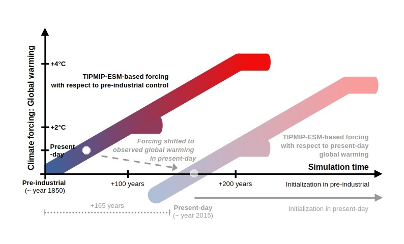
Models starting the experiments from a present-day as opposed to pre-industrial ice-sheet state (e.g. using an inversion method in the present-day for the model initialization) will not run the full ramp-up period and the forcing will be shifted accordingly. An example is described in Figure 2. Please contact us by e-mail in case of questions.
The ice-sheet modelling groups can choose how to translate these variables to the models, e.g. in terms of the surface mass balance or sub-shelf melt, depending on the approaches available for each model. More details as well as example approaches for the translation and respective references are provided below. We would like to stress that the lists of examples are not exclusive. Other approaches are welcome, and should be detailed in the README accompanying the submitted simulations (see README).
Atmospheric forcing
In TIPMIP-ICE SHEETS, the atmospheric forcing includes monthly near-surface air temperature anomalies and precipitation ratios (based on the CMIP variables tas and pr).
From near-surface air temperature and precipitation, the surface mass balance (defined as snowfall – rainfall – snow-melt – ice-melt + refreezing) should be calculated “online” by the participating ice-sheet models and as a function of the evolving ice-sheet geometry to capture the surface-melt elevation feedback, one of the key feedbacks associated with ice-sheet tipping dynamics in Greenland (Robinson et al., 2012; Petrini et al., 2025; Gutiérrez-González et al., 2026) and Antarctica (Garbe et al., 2020; Coulon et al., 2024). At the very least, the ESM-based near-surface air temperature (from Eq. 1) should be corrected for changes in the ice-sheet surface elevation during the simulation based on a spatially-uniform and time-independent atmospheric lapse rate (as in e.g. Coulon et al., 2024; Coulon/Klose et al., 2025), so that the “effective” near-surface air temperature reads as:
with the atmospheric lapse rate . We encourage the ice-sheet modelling groups to use alternative approaches, if available. A description of this approach has to be added in the provided README (see README).
Snow and ice melt should then be calculated using the adjusted air temperature, for example, using one of the following approaches:
- Positive-degree day approach (PDD) (e.g., Reeh, 1991; Calov and Greve, 2005; Coulon et al., 2024; Aschwanden et al., 2019)
- Simple diurnal Energy Balance Model (dEBM-simple) (e.g., Zeitz et al., 2021; Garbe et al., 2023)
- Insolation-Temperature-Melt (ITM) (e.g., Pellicciotti et al., 2005; van den Berg et al., 2008; Robinson et al., 2010)
Examples for determining the refreezing and thus runoff of surface meltwater include but are not limited to:
- Simple thermodynamic parameterisation of refreezing (e.g., Janssens and Huybrechts, 2000; Huybrechts and de Wolde, 1999; Tarasov and Peltier, 2002)
- Refreezing of constant fraction of surface melt (e.g., PISM Manual/Khrulev et al., 2026)
Ocean forcing
In TIPMIP-ICE SHEETS, the Antarctic ocean forcing includes annual mean ocean temperature and salinity anomalies (based on the CMIP variables thetao and so), which were extrapolated to the ice-shelf cavities and in currently ice-covered regions, based on the horizontal Gaussian extrapolation of Jourdain (2024). The Greenland ocean forcing is provided as monthly thermal forcing anomalies (based on the CMIP variables thetao and so). The calculation of the thermal forcing and the extrapolation of ocean properties into the fjords follows the approach of the ISMIP7 GIS Ocean Focus Group (Slater et al., in prep).
Sub-shelf melting and/or frontal melting should be calculated by the participating ice-sheet models based on ocean temperature and salinity.
For the Antarctic Ice Sheet, possible approaches for determining sub-shelf melting include, but are not limited to:
- Local quadratic parameterization (Favier et al., 2019; Burgard et al., 2022)
- ISMIP6 non-local quadratic parameterization (Jourdain et al., 2020)
- Potsdam Ice-shelf Cavity mOdel (PICO; Reese et al., 2018; Reese et al., 2023)
- Plume parameterization (Lazeroms et al., 2019)
- PICOP (Pelle et al., 2019), combining PICO and the plume parameterization
- LADDIE (Lambert et al., 2023)
Please also see Burgard et al. (2022), Coulon et al. (2024) and Lambert and Burgard (2025) for a comparison of common sub-shelf melt parameterizations and associated parameter ranges. While not required, frontal melt may be included in Antarctica.
For the Greenland Ice Sheet, possible approaches for determining frontal melting include, but are not limited to:
- ISMIP6 submarine melt implementation (Slater et al., 2020), determining frontal melt based on the parameterisation of Rignot et al. (2016) from subglacial discharge and thermal forcing. Note that the subglacial discharge may be based on the surface runoff determined by the participating ice-sheet models throughout the simulation (see Atmospheric forcing). Only the thermal forcing is provided in TIPMIP-ICE SHEETS (see Ocean forcing).
While not required, sub-shelf melt may be included in Greenland, e.g. based on one of the following approaches:
- Potsdam Ice-shelf Cavity mOdel (PICO; REF)
- Tunable present-day sub-shelf melt combined with linear, scaled anomalies (Tabone et al., 2024; Gutiérrez-González et al., 2026)
GIA
Given the crucial role of ice-sheet – solid Earth interactions for ice-sheet tipping dynamics (e.g. Gomez et al., 2010; Coulon et al., 2021; Zeitz et al., 2022), a representation of the response of the solid Earth to ice-sheet changes is required for participation in TIPMIP-ICE SHEETS. Examples include:
- Elastic lithosphere–relaxed asthenosphere (ELRA) model (Le Meur and Huybrechts, 1996)
- Laterally variable ELRA (LV-ELRA) model (Coulon et al., 2021)
- Elastic lithosphere–viscous mantel (ELVA) model (e.g., Lingle-Clark; Lingle and Clark, 1985; Bueler et al., 2007)
- LV-ELVA (e.g. FastIsostasy; Swierczek-Jereczek et al., 2024)
If available, more complex representations of ice-sheet – solid Earth interactions, e.g. including the laterally variable as well as radial structure of the solid Earth on a global domain (e.g., Albrecht et al., 2024), are welcome.
Calving
Changes in the ice-shelf front through calving have been an important driver in observed glacier speed-up in the Amundsen Sea over the past decades (De Rydt et al., 2021; dos Santos et al., 2021) and may determine the long-term stability of marine ice sheets (Haseloff and Sergienko, 2022). Similarly, calving rules have been shown to impact the steady states and the dynamic behavior of marine terminating glaciers (Sergienko, 2022; Schoof et al., 2017).
In ice-sheet models participating in TIPMIP-ICE SHEETS, the ice front should be free to retreat. Defining a maximum ice extent such that the ice sheet does not advance beyond e.g. its present-day configuration is allowed.
In Antarctica, calving at the ice-shelf front should be represented, for example, as
- Eigencalving (Levermann et al., 2012)
- Von Mises stress calving (Morlighem et al., 2016)
- Thickness calving / Minimum thickness threshold (as applied in, e.g., Garbe et al., 2020)
- Calving depending on surface/basal crevasse penetration depth (Pollard et al., 2015; DeConto and Pollard, 2016)
These calving laws have recently been assessed for Antarctic ice shelves (Wilner et al., 2023).
In Greenland, calving at the terminus of outlet glaciers should be included. Possible approaches include, but are not limited to
- Von Mises stress calving (Morlighem et al., 2016; Choi et al., 2017)
- Height-above buoyancy criterion (Vieli et al., 2001)
- Crevasse depth calving (Benn et al., 2017; Otero et al., 2010),
which have been compared by Amaral et al. (2020) and Choi et al. (2018) for various glaciers in Greenland.
README
Each participating ice-sheet modelling group has to submit a README file together with the submission of the simulations, following this template: [Note: README template will be added in the coming weeks.]
Output variables and file naming
TIPMIP-ICE SHEETS overall follows the conventions on the naming of ice-sheet model output variables and files from ISMIP7.
Requested ice-sheet model output variables
Table 3: Requested ice-sheet model output variables in TIPMIP-ICE SHEETS. ST and FL refer to “state variable” and “flux variable”, respectively. While ST variables should be submitted at the end of the modelled year, FL variables should be averaged over the respective year. In addition, time is recorded in different ways, depending on the variable type. Please see Format of ice-sheet model output files below for additional information on the time variable in the submitted file.
| Variable | Dim | Type | Variable name | Standard name | Unit | Mandatory | Comment |
| Ice thickness | x,y,t | ST | lithk | land_ice_thickness | m | y | Ice thickness of the ice sheet |
| Surface elevation | x,y,t | ST | orog | surface_altitude | m | y | Surface elevation of the ice sheet |
| Bedrock elevation | x,y,t | ST | topg | surface_altitude | m | y | Bedrock topography (may change during the projections) |
| Ice base elevation | x,y,t | ST | base | m | y | ||
| Geothermal heat flux | x,y,t | FL | hfgeoubed | upward_geothermal_heat_flux_in_land_ice | W m-2 | n | Geothermal heat flux at the ice interface |
| Surface mass balance flux | x,y,t | FL | acabf | land_ice_surface_specific_mass_balance_flux | kg m-2 s-1 | y | Surface mass balance flux |
| Basal mass balance flux beneath grounded ice | x,y,t | FL | libmassbfgr | land_ice_basal_specific_mass_balance_flux | kg m-2 s-1 | y | Basal mass balance flux (only beneath grounded ice) |
| Basal mass balance flux beneath floating ice | x,y,t | FL | libmassbffl | land_ice_basal_specific_mass_balance_flux | kg m-2 s-1 | y | Basal mass balance flux (only beneath floating ice) |
| Ice thickness imbalance | x,y,t | FL | dlithkdt | tendency_of_land_ice_thickness | m s-1 | y | dHdt |
| Surface velocity in x | x,y,t | ST | xvelsurf | land_ice_surface_x_velocity | m s-1 | n | u-velocity at land ice surface |
| Surface velocity in y | x,y,t | ST | yvelsurf | land_ice_surface_y_velocity | m s-1 | n | v-velocity at land ice surface |
| Surface velocity in z | x,y,t | ST | zvelsurf | land_ice_surface_upward_velocity | m s-1 | n | w-velocity at land ice surface |
| Basal velocity in x | x,y,t | ST | xvelbase | land_ice_basal_x_velocity | m s-1 | n | u-velocity at land ice base |
| Basal velocity in y | x,y,t | ST | yvelbase | land_ice_basal_y_velocity | m s-1 | n | v-velocity at land ice base |
| Basal velocity in z | x,y,t | ST | zvelbase | land_ice_basal_upward_velocity | m s-1 | n | w-velocity at land ice base |
| Mean velocity in x | x,y,t | ST | xvelmean | land_ice_vertical_mean_x_velocity | m s-1 | y | Vertical mean land ice velocity |
| Mean velocity in y | x,y,t | ST | yvelmean | land_ice_vertical_mean_y_velocity | m s-1 | y | Vertical mean land ice velocity is the average from the bedrock to the surface of the ice |
| Surface temperature | x,y,t | ST | litemptop | temperature_at_top_of_ice_sheet_model | K | n | Ice temperature at surface |
| Depth average temperature | x,y,t | ST | litempavg | K | n | ||
| Basal temperature beneath grounded ice sheet | x,y,t | ST | litempbotgr | temperature_at_base_of_ice_sheet_model | K | n | Ice temperature at base of grounded ice sheet |
| Basal temperature beneath floating ice shelf | x,y,t | ST | litempbotfl | temperature_at_base_of_ice_sheet_model | K | n | Ice temperature at base of grounded ice sheet |
| Basal drag | x,y,t | ST | strbasemag | land_ice_basal_drag | Pa | y | Basal drag |
| Calving flux | x,y,t | FL | licalvf | land_ice_specific_mass_flux_due_to_calving | kg m-2 s-1 | y | Ice mass change resulting from iceberg calving. Only for grid cells in contact with ocean |
| Grounding line flux | x,y,t | FL | ligroundf | kg m-2 s-1 | y | Flux of ice mass across the grounding line. Only for grounding line grid cells. | |
| Ice front melt flux | x,y,t | FL | lifmassbf | kg m-2 s-1 | y | Ice mass change resulting from ice front melting. Only for grid cells in contact with ocean. | |
| Land ice area fraction | x,y,t | ST | sftgif | land_ice_area_fraction | 1 | y | Fraction of grid cell covered by land ice |
| Grounded ice sheet area fraction | x,y,t | ST | sftgrf | grounded_ice_sheet_area_fraction | 1 | y | Fraction of grid cell covered by grounded ice sheet, where grounded indicates that the quantity correspond to the ice sheet that flows over bedrock |
| Floating ice sheet area fraction | x,y,t | ST | sftflf | floating_ice_shelf_area_fraction | 1 | y | Fraction of grid cell covered by ice sheet flowing over seawater |
| Thermal forcing at the ice base under floating ice shelves | x,y,t | ST | tfbase | K | n | Thermal forcing interpolated to the ice draft under floating ice shelves (fill value for purely grounded ice or not ice) | |
| Anomaly in geopotential height from reference geoid | x,y,t | ST | deltag | geopotential_height_anomaly | m | n | Change in geoid height should be relative to the reference geoid |
| Reference geoid | x,y | ST | refgeoid | geoid_height_above_reference_ellipsoid | m | n | Field is calculated with respect to the WGS84 reference ellipsoid |
| Ice temperature | x,y,z,t | ST | litemp | land_ice_temperature | K | n |
Format of ice-sheet model output files
Since simulations are based on a set of idealized experiments, the basetime in the submitted files should be 0000-1-1. Time should then be given as days since 0000-1-1 across the set of experiments (i.e. climate ramp-up, climate stabilization, climate reversal) with a 365_day calendar. Note that the ice-sheet model output should not be interpolated to this calendar. Instead, we will use a common time axis for the ice-sheet model output to facilitate the analysis. State variables should be given at the end of the modelled year, while flux variables are averaged over the respective year and recorded as the middle of the year. Please see the example in Table 4 below.
Ice-sheet model output should be submitted on the ISMIP grids, which are defined as follows:
- Greenland Ice Sheet: Polar stereographic projection with standard parallel at 70° N and central meridian of 45° W (315° E), referenced to WGS84 datum (EPSG:3413), Domain from (−720,000 m, −3,450,000 m)/lower-left corner to (960,000 m,−570,000 m)/upper-right corner
- Antarctic Ice Sheet: Polar stereographic projection with standard parallel at 71° S and central meridian of 0° W, referenced to WGS84 datum (EPSG:3031), Domain from (−3,040,000 m, −3,040,000 m)/lower-left corner to (3,040,000 m, 3,040,000 m)/upper-right corner
Table 4: Example for time variable in ice-sheet model output files. Time is given as days since 0000-1-1 with a 365_day calendar. Note that the length of the climate ramp-up experiments may slightly differ depending on the ESM. In addition, the example assumes that the climate stabilization and reversal experiments are run for 1000 years. Participating ice-sheet model groups are encouraged to further extend these experiments, if possible.
| State variable | Flux variable | |||||||||
| Year since initial state | Start | End | Entry in file | Time (in days since basetime) | Entry in file | Time (days since basetime + 0.5 years) | time_bnds (left) | time_bnds (right) | ||
| Climate ramp-up | ||||||||||
| 0 (Initial state) | 1/1/0000 | 1 | 0 | Initial state | ||||||
| 1 | 0000-1-1 | 0001-1-1 | 2 | 365 | value at end of 0000 | 1 | 365/2 | 0 | 365 | average for 0000 |
| 2 | 0001-1-1 | 0002-1-1 | 3 | 730 | value at end of 0001 | 2 | 365+182 | 365 | 730 | average for 0001 |
| … | … | … | … | … | … | … | … | … | … | … |
| 200 | 0200-1-1 | 0201-1-1 | 201 | 73000 | value at end of 200 | 200 | 72635+182 | 72635 | 73000 | average for 0200 |
| Climate stabilization | ||||||||||
| 201 | 0201-1-1 | 0202-1-1 | 1 | 73365 | value at end of 201 | 201 | 73000+182 | 73000 | 73365 | average over 201 |
| … | … | … | … | … | … | … | … | … | … | … |
| 1201 | 1201-1-1 | 1202-1-1 | 1000 | 438365 | value at end of 1201 | 1201 | 438000+182 | 438000 | 438365 | average over 1201 |
| Climate reversal | ||||||||||
| 1202 | 1202-1-1 | 1203-1-1 | 1 | 438730 | value at end of 1202 | 1202 | 438365+182 | 438365 | 438730 | average over 1202 |
| … | … | … | … | … | … | … | … | … | … | … |
| 2202 | 2202-1-1 | 2203-1-1 | 1000 | 803730 | value at end of 2202 | 2202 | 803415+182 | 803415 | 803730 | average over 1202 |
Naming of ice-sheet model output files
Each output variable listed in Table 3 should be submitted in a separate netcdf file, named as follows:
[variable]_[ice-sheet]_[modelling-group]_[ice-sheet-model]_[experiment-name].nc
For the naming of the experiment ([experiment-name]), please follow Table 1 and 2.
Data access and distribution
TIPMIP-ICE SHEETS data are stored at the German Climate Computing Centre (Deutsches Klimarechenzentrum, DKRZ). A DKRZ account is required for (1) downloading the forcing (input) data (Klose et al., in prep.), and (2) uploading the ice-sheet model (output) data. Please contact data@tipmip.org and icesheets@tipmip.org in both cases for detailed instructions.
Acknowledgements
- We gratefully acknowledge the work of the Ice Sheet Model Intercomparison Project (ISMIP) and their Focus Groups for establishing a number of methods and common practices for community ice-sheet modelling that we have adapted and made use of for TIPMIP-ICE SHEETS.
- We thank the Earth System modelling groups participating in TIPMIP-ESM for producing and making their model output available to TIPMIP-ICE SHEETS, which have formed the basis for constructing the forcing for the standalone ice-sheet model experiments.
- We thank the participating ice-sheet modelling groups for their commitment to TIPMIP-ICE SHEETS including their contributions to the experimental protocol as well as the submissions of simulations.
- We thank all colleagues of the wider TIPMIP community, attending the various domain workshops, the WE-Heraeus Seminar on ‘Addressing Key Uncertainties in Modelling Physical and Ecological Tipping Dynamics in the Earth System’ in Templin (Germany, 2023), the TIPMIP General Assemblies in Baltimore (US, 2024) and in Tokyo (Japan, 2026) for fruitful discussions on the experimental design.
Appendix: Shifting forcing
Table 5: Observed and simulated global surface temperature change above pre-industrial. Observed global surface temperature change is based on the Copernicus Climate Change Service Global Indicators Temperature Dataset (Copernicus Climate Change Service, 2026). The simulated global surface temperature change is based on the TIPMIP-ESM ramp-up simulation by NorESM2-LM and UKESM1-2-LL, chosen as Tier 1 ESMs for the Antarctic and Greenland ice sheets, respectively. Assuming the initial Antarctic ice-sheet state is associated with e.g. the year 2015 with an observed global warming of 0.98 °C above pre-industrial levels (left columns, marked in bold), this ice-sheet model would only consider the TIPMIP-ESM-based ramp-up from the ESM simulation year 56 / 45 onwards (beyond which global warming does not fall below 0.98 °C in the TIPMIP-ESM-based forcing, right columns, marked in bold) in simulations for the Antarctic / Greenland ice sheets. The TIPMIP-ESM-based forcing would be shifted with respect to the simulation year 56 / 45 (passing through zero at the start of the ice-sheet’s model ramp up) in simulations for the Antarctic / Greenland ice sheets.
| Year | Observed global surface temperature change | TIPMIP-ESM simulation time | Simulated global surface temperature change in TIPMIP-ESM ramp-up from NorESM2-LM (Tier 1 ESM for Antarctic Ice Sheet) | Simulated global surface temperature change in TIPMIP-ESM ramp-up from UKESM1-2-LL (Tier 1 ESM for Greenland Ice Sheet) |
| 1850 | 1 | |||
| 1851 | 2 | |||
| 1852 | 3 | |||
| 1853 | 4 | |||
| 1854 | 0.08 | 5 | 0.19 | -0.06 |
| 1855 | 0.11 | 6 | 0.18 | -0.03 |
| 1856 | 0.09 | 7 | 0.17 | -0.05 |
| 1857 | 0.05 | 8 | 0.17 | -0.05 |
| 1858 | 0.03 | 9 | 0.2 | -0.01 |
| 1859 | 0.03 | 10 | 0.27 | 0.06 |
| 1860 | 0.01 | 11 | 0.33 | 0.11 |
| 1861 | -0.01 | 12 | 0.36 | 0.17 |
| 1862 | -0.03 | 13 | 0.33 | 0.23 |
| 1863 | -0.03 | 14 | 0.29 | 0.27 |
| 1864 | -0.07 | 15 | 0.22 | 0.28 |
| 1865 | -0.05 | 16 | 0.19 | 0.34 |
| 1866 | -0.02 | 17 | 0.24 | 0.39 |
| 1867 | 0.02 | 18 | 0.33 | 0.4 |
| 1868 | 0.03 | 19 | 0.43 | 0.43 |
| 1869 | 0.07 | 20 | 0.52 | 0.45 |
| 1870 | 0.06 | 21 | 0.6 | 0.44 |
| 1871 | 0.05 | 22 | 0.62 | 0.46 |
| 1872 | 0.06 | 23 | 0.66 | 0.46 |
| 1873 | 0.05 | 24 | 0.67 | 0.5 |
| 1874 | 0.03 | 25 | 0.67 | 0.53 |
| 1875 | 0.02 | 26 | 0.66 | 0.53 |
| 1876 | 0.01 | 27 | 0.67 | 0.51 |
| 1877 | 0.06 | 28 | 0.65 | 0.55 |
| 1878 | 0.13 | 29 | 0.75 | 0.54 |
| 1879 | 0.15 | 30 | 0.81 | 0.57 |
| 1880 | 0.16 | 31 | 0.81 | 0.64 |
| 1881 | 0.2 | 32 | 0.78 | 0.69 |
| 1882 | 0.15 | 33 | 0.77 | 0.74 |
| 1883 | 0.09 | 34 | 0.74 | 0.78 |
| 1884 | 0.05 | 35 | 0.77 | 0.81 |
| 1885 | 0.03 | 36 | 0.81 | 0.82 |
| 1886 | -0.02 | 37 | 0.85 | 0.86 |
| 1887 | -0.06 | 38 | 0.9 | 0.88 |
| 1888 | -0.06 | 39 | 0.88 | 0.91 |
| 1889 | -0.01 | 40 | 0.88 | 0.95 |
| 1890 | -0.02 | 41 | 0.92 | 0.94 |
| 1891 | 0 | 42 | 0.94 | 0.95 |
| 1892 | 0.01 | 43 | 0.93 | 0.95 |
| 1893 | -0.02 | 44 | 0.95 | 0.97 |
| 1894 | -0.07 | 45 | 0.92 | 1 |
| 1895 | -0.05 | 46 | 0.9 | 1.02 |
| 1896 | -0.03 | 47 | 0.91 | 1.04 |
| 1897 | 0.01 | 48 | 0.92 | 1.06 |
| 1898 | 0.02 | 49 | 0.92 | 1.07 |
| 1899 | 0.05 | 50 | 0.95 | 1.1 |
| 1900 | 0.09 | 51 | 0.95 | 1.14 |
| 1901 | 0.08 | 52 | 0.93 | 1.15 |
| 1902 | 0.05 | 53 | 0.95 | 1.15 |
| 1903 | 0.03 | 54 | 0.93 | 1.16 |
| 1904 | -0.03 | 55 | 0.94 | 1.16 |
| 1905 | -0.07 | 56 | 1 | 1.19 |
| 1906 | -0.08 | 57 | 1.04 | 1.21 |
| 1907 | -0.1 | 58 | 1.09 | 1.22 |
| 1908 | -0.1 | 59 | 1.18 | 1.22 |
| 1909 | -0.1 | 60 | 1.19 | 1.22 |
| 1910 | -0.12 | 61 | 1.19 | 1.24 |
| 1911 | -0.17 | 62 | 1.22 | 1.32 |
| 1912 | -0.17 | 63 | 1.2 | 1.34 |
| 1913 | -0.15 | 64 | 1.17 | 1.34 |
| 1914 | -0.09 | 65 | 1.21 | 1.36 |
| 1915 | -0.03 | 66 | 1.26 | 1.3 |
| 1916 | -0.01 | 67 | 1.3 | 1.26 |
| 1917 | -0.03 | 68 | 1.39 | 1.28 |
| 1918 | -0.02 | 69 | 1.45 | 1.28 |
| 1919 | -0.04 | 70 | 1.44 | 1.29 |
| 1920 | -0.07 | 71 | 1.4 | 1.37 |
| 1921 | -0.03 | 72 | 1.4 | 1.43 |
| 1922 | 0.01 | 73 | 1.41 | 1.48 |
| 1923 | 0.03 | 74 | 1.42 | 1.52 |
| 1924 | 0.03 | 75 | 1.44 | 1.55 |
| 1925 | 0.04 | 76 | 1.48 | 1.55 |
| 1926 | 0.06 | 77 | 1.49 | 1.58 |
| 1927 | 0.08 | 78 | 1.49 | 1.64 |
| 1928 | 0.1 | 79 | 1.47 | 1.7 |
| 1929 | 0.08 | 80 | 1.41 | 1.7 |
| 1930 | 0.1 | 81 | 1.39 | 1.71 |
| 1931 | 0.1 | 82 | 1.42 | 1.74 |
| 1932 | 0.11 | 83 | 1.46 | 1.75 |
| 1933 | 0.1 | 84 | 1.51 | 1.76 |
| 1934 | 0.14 | 85 | 1.65 | 1.78 |
| 1935 | 0.13 | 86 | 1.78 | 1.78 |
| 1936 | 0.12 | 87 | 1.83 | 1.75 |
| 1937 | 0.15 | 88 | 1.78 | 1.74 |
| 1938 | 0.21 | 89 | 1.76 | 1.77 |
| 1939 | 0.23 | 90 | 1.79 | 1.83 |
| 1940 | 0.28 | 91 | 1.78 | 1.85 |
| 1941 | 0.33 | 92 | 1.75 | 1.88 |
| 1942 | 0.33 | 93 | 1.81 | 1.9 |
| 1943 | 0.33 | 94 | 1.92 | 1.89 |
| 1944 | 0.36 | 95 | 1.93 | 1.9 |
| 1945 | 0.35 | 96 | 1.92 | 1.96 |
| 1946 | 0.32 | 97 | 1.98 | 1.98 |
| 1947 | 0.31 | 98 | 2.04 | 1.97 |
| 1948 | 0.29 | 99 | 2.08 | 2 |
| 1949 | 0.23 | 100 | 2.11 | 2.01 |
| 1950 | 0.19 | 101 | 2.08 | 2.02 |
| 1951 | 0.19 | 102 | 2.02 | 2.06 |
| 1952 | 0.2 | 103 | 2.03 | 2.12 |
| 1953 | 0.24 | 104 | 2.01 | 2.19 |
| 1954 | 0.23 | 105 | 1.98 | 2.17 |
| 1955 | 0.24 | 106 | 2 | 2.19 |
| 1956 | 0.2 | 107 | 2.1 | 2.21 |
| 1957 | 0.21 | 108 | 2.12 | 2.19 |
| 1958 | 0.2 | 109 | 2.1 | 2.18 |
| 1959 | 0.23 | 110 | 2.18 | 2.21 |
| 1960 | 0.25 | 111 | 2.24 | 2.21 |
| 1961 | 0.3 | 112 | 2.2 | 2.22 |
| 1962 | 0.3 | 113 | 2.11 | 2.29 |
| 1963 | 0.29 | 114 | 2.09 | 2.31 |
| 1964 | 0.25 | 115 | 2.13 | 2.33 |
| 1965 | 0.23 | 116 | 2.15 | 2.39 |
| 1966 | 0.21 | 117 | 2.27 | 2.38 |
| 1967 | 0.2 | 118 | 2.4 | 2.34 |
| 1968 | 0.18 | 119 | 2.43 | 2.36 |
| 1969 | 0.23 | 120 | 2.37 | 2.41 |
| 1970 | 0.25 | 121 | 2.43 | 2.41 |
| 1971 | 0.24 | 122 | 2.41 | 2.44 |
| 1972 | 0.25 | 123 | 2.32 | 2.49 |
| 1973 | 0.29 | 124 | 2.34 | 2.49 |
| 1974 | 0.26 | 125 | 2.44 | 2.47 |
| 1975 | 0.25 | 126 | 2.47 | 2.5 |
| 1976 | 0.24 | 127 | 2.51 | 2.52 |
| 1977 | 0.27 | 128 | 2.6 | 2.55 |
| 1978 | 0.25 | 129 | 2.66 | 2.56 |
| 1979 | 0.31 | 130 | 2.58 | 2.61 |
| 1980 | 0.37 | 131 | 2.52 | 2.67 |
| 1981 | 0.46 | 132 | 2.53 | 2.68 |
| 1982 | 0.46 | 133 | 2.53 | 2.67 |
| 1983 | 0.51 | 134 | 2.44 | 2.71 |
| 1984 | 0.5 | 135 | 2.44 | 2.77 |
| 1985 | 0.47 | 136 | 2.49 | 2.76 |
| 1986 | 0.44 | 137 | 2.51 | 2.81 |
| 1987 | 0.48 | 138 | 2.53 | 2.86 |
| 1988 | 0.49 | 139 | 2.68 | 2.88 |
| 1989 | 0.52 | 140 | 2.79 | 2.87 |
| 1990 | 0.58 | 141 | 2.85 | 2.91 |
| 1991 | 0.63 | 142 | 2.88 | 2.91 |
| 1992 | 0.6 | 143 | 2.86 | 2.94 |
| 1993 | 0.58 | 144 | 2.78 | 2.98 |
| 1994 | 0.59 | 145 | 2.76 | 2.99 |
| 1995 | 0.59 | 146 | 2.78 | 2.98 |
| 1996 | 0.58 | 147 | 2.77 | 3.03 |
| 1997 | 0.63 | 148 | 2.83 | 3.07 |
| 1998 | 0.71 | 149 | 2.96 | 3.09 |
| 1999 | 0.73 | 150 | 2.99 | 3.12 |
| 2000 | 0.71 | 151 | 2.97 | 3.15 |
| 2001 | 0.75 | 152 | 3 | 3.17 |
| 2002 | 0.78 | 153 | 3.04 | 3.16 |
| 2003 | 0.78 | 154 | 3.03 | 3.16 |
| 2004 | 0.81 | 155 | 3.12 | 3.19 |
| 2005 | 0.87 | 156 | 3.22 | 3.21 |
| 2006 | 0.89 | 157 | 3.24 | 3.24 |
| 2007 | 0.89 | 158 | 3.21 | 3.25 |
| 2008 | 0.88 | 159 | 3.23 | 3.29 |
| 2009 | 0.9 | 160 | 3.24 | 3.3 |
| 2010 | 0.91 | 161 | 3.2 | 3.3 |
| 2011 | 0.9 | 162 | 3.22 | 3.28 |
| 2012 | 0.9 | 163 | 3.34 | 3.28 |
| 2013 | 0.93 | 164 | 3.39 | 3.29 |
| 2014 | 0.95 | 165 | 3.29 | 3.28 |
| 2015 | 0.98 | 166 | 3.23 | 3.28 |
| 2016 | 1.06 | 167 | 3.23 | 3.29 |
| 2017 | 1.12 | 168 | 3.21 | 3.29 |
| 2018 | 1.15 | 169 | 3.24 | 3.29 |
| 2019 | 1.2 | 170 | 3.31 | 3.34 |
| 2020 | 1.22 | 171 | 3.35 | 3.33 |
| 2021 | 1.19 | 172 | 3.35 | 3.34 |
| 2022 | 1.18 | 173 | 3.36 | 3.37 |
| 2023 | 1.25 | 174 | 3.37 | 3.39 |
| 2024 | 1.31 | 175 | 3.37 | 3.38 |
| 2025 | 1.34 | 176 | 3.42 | 3.46 |
| 177 | 3.5 | 3.52 | ||
| 178 | 3.52 | 3.51 | ||
| 179 | 3.48 | 3.52 | ||
| 180 | 3.55 | 3.57 | ||
| 181 | 3.61 | 3.56 | ||
| 182 | 3.56 | 3.58 | ||
| 183 | 3.54 | 3.69 | ||
| 184 | 3.56 | 3.73 | ||
| 185 | 3.52 | 3.76 | ||
| 186 | 3.45 | 3.82 | ||
| 187 | 3.46 | 3.85 | ||
| 188 | 3.48 | 3.82 | ||
| 189 | 3.55 | 3.81 | ||
| 190 | 3.62 | 3.82 | ||
| 191 | 3.68 | 3.81 | ||
| 192 | 3.75 | 3.82 | ||
| 193 | 3.81 | 3.83 | ||
| 194 | 3.78 | 3.86 | ||
| 195 | 3.78 | |||
| 196 | 3.85 | |||
| 197 | 3.86 | |||
| 198 | 3.82 | |||
| 199 | 3.85 | |||
| 200 | 3.86 | |||
| 201 | 3.81 | |||
| 202 | 3.78 | |||
| 203 | 3.81 | |||
| 204 | 3.83 | |||
| 205 | 3.88 | |||
| 206 | 3.95 | |||
| 207 | 4.06 |
References
Albrecht, T., Bagge, M., and Klemann, V. (2024): Feedback mechanisms controlling Antarctic glacial-cycle dynamics simulated with a coupled ice sheet–solid Earth model, The Cryosphere, 18, 4233–4255, https://doi.org/10.5194/tc-18-4233-2024.
Amaral, T., Bartholomaus, T. C., and Enderlin, E. M. (2020): Evaluation of iceberg calving models against observations from Greenland outlet glaciers. Journal of Geophysical Research: Earth Surface, 125, e2019JF005444, https://doi.org/10.1029/2019JF005444.
Aschwanden, A., Fahnestock, M. A., Truffer, M., Brinkerhoff, D. J., Hock, R., Khroulev, C., … & Khan, S. A. (2019): Contribution of the Greenland Ice Sheet to sea level over the next millennium, Science Advances, 5(6), eaav9396, https://doi.org/10.1126/sciadv.aav9396.
Bueler, E., Lingle, C. S., and Brown, J. (2007): Fast computation of a viscoelastic deformable Earth model for ice-sheet simulations, Annals of Glaciology, 46, 97–105, https://doi.org/10.3189/172756407782871567.
Burgard, C., Jourdain, N. C., Reese, R., Jenkins, A., and Mathiot, P. (2022): An assessment of basal melt parameterisations for Antarctic ice shelves, The Cryosphere, 16, 4931–4975, https://doi.org/10.5194/tc-16-4931-2022.
Calov, R. and Greve, R. (2005): A semi-analytical solution for the positive degree-day model with stochastic temperature variations, Journal of Glaciologz, 51, 173–175, https://doi.org/10.3189/172756505781829601.
Choi, Y., Morlighem, M., Rignot, E., Mouginot, J., and Wood, M. (2017): Modeling the response of Nioghalvfjerdsfjorden and Zachariae Isstrøm glaciers, Greenland, to ocean forcing over the next century, Geophysical Research Letters, 44, 11071–11079, https://doi.org/10.1002/2017GL075174.
Choi, Y., Morlighem, M., Wood, M., and Bondzio, J. H. (2018): Comparison of four calving laws to model Greenland outlet glaciers, The Cryosphere, 12, 3735–3746, https://doi.org/10.5194/tc-12-3735-2018.
Copernicus Climate Change Service (2026): Climate Indicators Temperature, https://climate.copernicus.eu/climate-indicators/temperature, last access: 12 July 2026.
Coulon, V., Bulthuis, K., Whitehouse, P. L., Sun, S., Haubner, K., Zipf, L., and Pattyn, F. (2021): Contrasting response of West and East Antarctic ice sheets to glacial isostatic adjustment, Journal of Geophysical Research: Earth Surface, 126, e2020JF006003, https://doi.org/10.1029/2020JF006003.
Coulon, V., Klose, A. K., Kittel, C., Edwards, T., Turner, F., Winkelmann, R., and Pattyn, F. (2024): Disentangling the drivers of future Antarctic ice loss with a historically calibrated ice-sheet model, The Cryosphere, 18, 653–681, https://doi.org/10.5194/tc-18-653-2024.
DeConto, R. M. and Pollard, D. (2016): Contribution of Antarctica to past and future sea-level rise, Nature, 531, 591–597, https://doi.org/10.1038/nature17145.
De Rydt, J., Reese, R., Paolo, F. S., and Gudmundsson, G. H. (2021): Drivers of Pine Island Glacier speed-up between 1996 and 2016, The Cryosphere, 15, 113–132, https://doi.org/10.5194/tc-15-113-2021.
Favier, L., Jourdain, N. C., Jenkins, A., Merino, N., Durand, G., Gagliardini, O., Gillet-Chaulet, F., and Mathiot, P. (2019): Assessment of sub-shelf melting parameterisations using the ocean–ice-sheet coupled model NEMO(v3.6)–Elmer/Ice(v8.3) , Geoscientific Model Development, 12, 2255–2283, https://doi.org/10.5194/gmd-12-2255-2019.
Garbe, J., Albrecht, T., Levermann, A., Donges, J. F., and Winkelmann, R. (2020): The hysteresis of the Antarctic Ice Sheet, Nature, 585, 538–544, https://doi.org/10.1038/s41586-020-2727-5.
Garbe, J., Zeitz, M., Krebs-Kanzow, U., and Winkelmann, R. (2023): The evolution of future Antarctic surface melt using PISM-dEBM-simple, The Cryosphere, 17, 4571–4599, https://doi.org/10.5194/tc-17-4571-2023.
Gomez, N., Mitrovica, J. X., Huybers, P., and Clark, P. U. (2010): Sea level as a stabilizing factor for marine-ice-sheet grounding lines, Nature Geoscience, 3, 850-853, https://doi.org/10.1038/ngeo1012.
Gutiérrez-González, L., Robinson, A., Alvarez-Solas, J., Tabone, I., Swierczek-Jereczek, J., Moreno-Parada, D., and Montoya, M. (2026): Hysteresis of the Greenland ice sheet from the Last Glacial Maximum to the future, The Cryosphere, 20(2), 1139-1162, https://doi.org/10.5194/tc-20-1139-2026.
Haseloff, M., and Sergienko, O.V. (2022): Effects of calving and submarine melting on steady states and stability of buttressed marine ice sheets, Journal of Glaciology, 68, 1149-1166, https://doi.org/10.1017/jog.2022.29.
Huybrechts, P., and de Wolde, J. (1999): The Dynamic Response of the Greenland and Antarctic Ice Sheets to Multiple-Century Climatic Warming, Journal of Climate, 12, 2169–2188.
Janssens, I. and Huybrechts, P. (2000): The treatment of meltwater retention in Mass-balance parameterisation of the Greenland Ice Sheet, Annals of Glaciology, 31, 133–140, https://doi.org/10.3189/172756400781819941.
Jones, C., Bossert, I., Dennis, D. P., Jeffery, H., Jones, C. D., Koenigk, T., Loriani, S., Sanderson, B., Séférian, R., Wyser, K., Yang, S., Abe, M., Bathiany, S., Braconnot, P., Brovkin, V., Burger, F. A., Cadule, P., Castruccio, F. S., Danabasoglu, G., Dittus, A., Donges, J. F., Fröb, F., Frölicher, T., Georgievski, G., Guo, C., Hu, A., Lawrence, P., Lerner, P., Licón-Saláiz, J., Otto-Bliesner, B., Romanou, A., Shevliakova, E., Silvy, Y., Swingedouw, D., Tjiputra, J., Walton, J., Wiltshire, A., Winkelmann, R., Wood, R., Yokohata, T., and Ziehn, T. (in review): The TIPMIP Earth system model experiment protocol: phase 1, https://doi.org/10.5194/egusphere-2025-3604.
Jourdain, N. C. (2024): nicojourdain/CMIP6_data_to_ISMIP6_grid: v1.0 (v1.0). Zenodo. https://doi.org/10.5281/zenodo.12755910.
Jourdain, N. C., Asay-Davis, X., Hattermann, T., Straneo, F., Seroussi, H., Little, C. M., and Nowicki, S. (2020): A protocol for calculating basal melt rates in the ISMIP6 Antarctic ice sheet projections, The Cryosphere, 14, 3111–3134, https://doi.org/10.5194/tc-14-3111-2020.
Khrulev, C., Aschwanden, A., Bueler, E., Brown, J., Maxwell, D., Albrecht, T., Reese, R., Mengel, M., Martin, M., Winkelmann, R., Zeitz, M., Levermann, A., Feldmann, J., Garbe, J., Haseloff, M., Seguinot, J., Hinck, S., Kleiner, T., Fischer, E., … Schoell, S. (2026): Parallel Ice Sheet Model (PISM) (v2.2.4). Zenodo. https://doi.org/10.5281/zenodo.19443904.
Klose, A. K., Coulon, V., Pattyn, F., and Winkelmann, R. (2024): The long-term sea-level commitment from Antarctica, The Cryosphere, 18, 4463–4492, https://doi.org/10.5194/tc-18-4463-2024.
Klose et al. (in prep.): Ice-sheet model forcings for exploring tipping dynamics in Greenland and Antarctica in TIPMIP-ICE SHEETS.
Lambert, E. and Burgard, C. (2025): Brief communication: Sensitivity of Antarctic ice shelf melting to ocean warming across basal melt models, The Cryosphere, 19, 2495–2505, https://doi.org/10.5194/tc-19-2495-2025.
Lambert, E., Jüling, A., van de Wal, R. S. W., and Holland, P. R. (2023): Modelling Antarctic ice shelf basal melt patterns using the one-layer Antarctic model for dynamical downscaling of ice–ocean exchanges (LADDIE v1.0), The Cryosphere, 17, 3203–3228, https://doi.org/10.5194/tc-17-3203-2023.
Lazeroms, W. M. J., Jenkins, A., Gudmundsson, G. H., and van de Wal, R. S. W. (2018): Modelling present-day basal melt rates for Antarctic ice shelves using a parametrization of buoyant meltwater plumes, The Cryosphere, 12, 49–70, https://doi.org/10.5194/tc-12-49-2018.
Le Meur, E. and Huybrechts, P. (1996): A comparison of different ways of dealing with isostasy: examples from modelling the Antarctic ice sheet during the last glacial cycle, Annals of Glaciology, 23, 309–317, https://doi.org/10.3189/S0260305500013586.
Levermann, A., Albrecht, T., Winkelmann, R., Martin, M. A., Haseloff, M., and Joughin, I. (2012): Kinematic first-order calving law implies potential for abrupt ice-shelf retreat, The Cryosphere, 6, 273–286, https://doi.org/10.5194/tc-6-273-2012.
Lingle, C. S. and Clark, J. A. (1985): A numerical model of interactions between a marine ice sheet and the solid earth: Application to a West Antarctic ice stream, Journal of Geophysical Research: Oceans, 90, 1100–1114, https://doi.org/10.1029/JC090iC01p01100,.
Morlighem, M., Bondzio, J., Seroussi, H., Rignot, E., Larour, E., Humbert, A. and Rebuffi, S. (2016): Modeling of Store Gletscher’s calving dynamics, West Greenland, in response to ocean thermal forcing, Geophysical Research Letters, 43, 2659–2666, https://doi.org/10.1002/2016GL067695.
Pellicciotti, F., Brock, B., Strasser, U., Burlando, P., Funk, M., and Corripio, J. (2005): An enhanced temperature-index glacier melt model including the shortwave radiation balance: development and testing for Haut Glacier d’Arolla, Switzerland, Journal of Glaciology, 51, 573–587, https://doi.org/10.3189/172756505781829124.
Pelle, T., Morlighem, M., and Bondzio, J. H. (2019): Brief communication: PICOP, a new ocean melt parameterization under ice shelves combining PICO and a plume model, The Cryosphere, 13, 1043–1049, https://doi.org/10.5194/tc-13-1043-2019.
Petrini, M., Scherrenberg, M. D. W., Muntjewerf, L., Vizcaino, M., Sellevold, R., Leguy, G. R., Lipscomb, W. H., and Goelzer, H. (2025): A topographically controlled tipping point for complete Greenland ice sheet melt, The Cryosphere, 19, 63–81, https://doi.org/10.5194/tc-19-63-2025.
Pollard, D., DeConto, R. M., and Alley, R. B. (2015): Potential Antarctic Ice Sheet retreat driven by hydrofracturing and ice cliff failure, Earth and Planetary Science Letters, 412, 112–121, https://doi.org/10.1016/j.epsl.2014.12.035.
Reeh, N. (1991): Parameterization of melt rate and surface temperature on the Greenland ice sheet, Polarforschung, 59, 113–128.
Reese, R., Albrecht, T., Mengel, M., Asay-Davis, X., and Winkelmann, R. (2018): Antarctic sub-shelf melt rates via PICO, The Cryosphere, 12, 1969–1985, https://doi.org/10.5194/tc-12-1969-2018.
Reese, R., Garbe, J., Hill, E. A., Urruty, B., Naughten, K. A., Gagliardini, O., Durand, G., Gillet-Chaulet, F., Gudmundsson, G. H., Chandler, D., Langebroek, P. M., and Winkelmann, R. (2023): The stability of present-day Antarctic grounding lines – Part 2: Onset of irreversible retreat of Amundsen Sea glaciers under current climate on centennial timescales cannot be excluded, The Cryosphere, 17, 3761–3783, https://doi.org/10.5194/tc-17-3761-2023.
Rignot, E., Xu, Y., Menemenlis, D., Mouginot, J., Scheuchl, B., Li, X., Morlighem, M., Seroussi, H., den Broeke, M. v., Fenty, I., Cai, C., An, L., and Fleurian, B. d. (2016): Modeling of ocean-induced ice melt rates of five west Greenland glaciers over the past two decades, Geophysical Research Letters, 43, 6374–6382, https://doi.org/10.1002/2016GL068784.
Rignot, E., Scheuchl, B., Barre, J.B., Brancato, V., Charrier, L., Chen, H., Ciraci, E., Dinh, A., Herreid, S., Jeong, S., Li, X., Mitchell, T., Mohajerani, Y., Shamsian, S., Tolpekin, V., Velicogna, I., and Wollersheim, M. (2026): Thirty years of glacier grounding line retreat in Antarctica, Proceedings of the National Academy of Sciences of the United States of America, 123 (10) e2524380123, https://doi.org/10.1073/pnas.2524380123.
Robinson, A., Calov, R., and Ganopolski, A. (2010): An efficient regional energy-moisture balance model for simulation of the Greenland Ice Sheet response to climate change, The Cryosphere, 4, 129–144, https://doi.org/10.5194/tc-4-129-2010.
Robinson, A., Calov, R., and Ganopolski, A. (2012): Multistability and critical thresholds of the Greenland ice sheet, Nature Climate Change, 2, 429–432, https://doi.org/10.1038/nclimate1449.
Röntgen et al. (in prep.): Exploring changes in the polar regions in TIPMIP-Earth System Models.
dos Santos, T. D., Barnes, J. M., Goldberg, D. N., Gudmundsson, G. H., and Morlighem, M. (2021): Drivers of change of Thwaites Glacier, West Antarctica, between 1995 and 2015. Geophysical Research Letters, 48, e2021GL093102, https://doi.org/10.1029/2021GL093102.
Schoof, C., Davis, A. D., and Popa, T. V. (2017): Boundary layer models for calving marine outlet glaciers, The Cryosphere, 11, 2283–2303, https://doi.org/10.5194/tc-11-2283-2017.
Sergienko, O. V. (2022): Marine outlet glacier dynamics, steady states and steady-state stability. Journal of Glaciology, 68(271), 946–960, https://doi.org/10.1017/jog.2022.13.
Slater, D. A., Felikson, D., Straneo, F., Goelzer, H., Little, C. M., Morlighem, M., Fettweis, X., and Nowicki, S. (2020): Twenty-first century ocean forcing of the Greenland ice sheet for modelling of sea level contribution, The Cryosphere, 14, 985–1008, https://doi.org/10.5194/tc-14-985-2020.
Swierczek-Jereczek, J., Montoya, M., Latychev, K., Robinson, A., Alvarez-Solas, J., and Mitrovica, J. (2024): FastIsostasy v1.0 – a regional, accelerated 2D glacial isostatic adjustment (GIA) model accounting for the lateral variability of the solid Earth, Geoscientific Model Development, 17, 5263–5290, https://doi.org/10.5194/gmd-17-5263-2024.
Tabone, I., Robinson, A., Montoya, M., & Alvarez-Solas, J. (2024): Holocene thinning in central Greenland controlled by the Northeast Greenland Ice Stream, Nature Communications, 15(1), 6434, https://doi.org/10.1038/s41467-024-50772-5.
Tarasov, L., Peltier, W. R. (2002): Greenland glacial history and local geodynamic consequences, Geophysical Journal International, 150(1), 198–229, https://doi.org/10.1046/j.1365-246X.2002.01702.x.
van den Berg, J., van de Wal, R., and Oerlemans, H. (2008): A mass balance model for the Eurasian Ice Sheet for the last 120,000 years, Global and Planetary Change, 61, 194–208, https://doi.org/10.1016/j.gloplacha.2007.08.015.
Wilner, J. A., Morlighem, M., and Cheng, G. (2023): Evaluation of four calving laws for Antarctic ice shelves, The Cryosphere, 17, 4889–4901, https://doi.org/10.5194/tc-17-4889-2023.
Winkelmann, R., Dennis, D. P., Donges, J. F., Loriani, S., Klose, A. K., Abrams, J. F., Alvarez-Solas, J., Albrecht, T., Armstrong McKay, D., Bathiany, S., Blasco Navarro, J., Brovkin, V., Burke, E., Danabasoglu, G., Donner, R. V., Drüke, M., Georgievski, G., Goelzer, H., Harper, A. B., Hegerl, G., Hirota, M., Hu, A., Jackson, L. C., Jones, C., Kim, H., Koenigk, T., Lawrence, P., Lenton, T. M., Liddy, H., Licón-Saláiz, J., Menthon, M., Montoya, M., Nitzbon, J., Nowicki, S., Otto-Bliesner, B., Pausata, F., Rahmstorf, S., Ramin, K., Robinson, A., Rockström, J., Romanou, A., Sakschewski, B., Schädel, C., Sherwood, S., Smith, R. S., Steinert, N. J., Swingedouw, D., Willeit, M., Weijer, W., Wood, R., Wyser, K., and Yang, S.: The Tipping Points Modelling Intercomparison Project (TIPMIP) (in review): Assessing tipping point risks in the Earth system, https://doi.org/10.5194/egusphere-2025-1899.
Winkelmann, R.*/Klose, A.K.* et al. (in prep.): TIPMIP-ICE SHEETS: Experimental design and pilot experiments. *Contributed equally to this work.
Zeitz, M., Reese, R., Beckmann, J., Krebs-Kanzow, U., and Winkelmann, R. (2021): Impact of the melt–albedo feedback on the future evolution of the Greenland Ice Sheet with PISM-dEBM-simple, The Cryosphere, 15, 5739–5764, https://doi.org/10.5194/tc-15-5739-2021.
Zeitz, M., Haacker, J. M., Donges, J. F., Albrecht, T., and Winkelmann, R. (2022): Dynamic regimes of the Greenland Ice Sheet emerging from interacting melt–elevation and glacial isostatic adjustment feedbacks, Earth System Dynamics, 13, 1077–1096, https://doi.org/10.5194/esd-13-1077-2022.